6 Options Trading Strategies and Hedging

References

HULL, John. Options, futures, and other derivatives. Ninth edition. Harlow: Pearson, 2018. ISBN 978-1-292-21289-0.
- Chapter 12 - Trading Strategies Involving Options
PIRIE, Wendy L. Derivatives. Hoboken: Wiley, 2017. CFA institute investment series. ISBN 978-1-119-38181-5.
- Chapter 5 - Derivatives Strategies

Additonal sources on option trading strategies:

Learning Outcomes:

Understand the structure and purpose of Principal Protected Notes, including how they safeguard the principal amount while offering potential investment gains.
Analyze strategies that combine positions in the underlying asset with options to manage risk and enhance potential returns, focusing on protective puts and covered calls.
Explore various option spread strategies, such as bull spreads, bear spreads, calendar spreads, and butterfly spreads, to understand their risk/reward profiles and market outlook implications.
Examine option combination strategies like straddles, strangles, strips, and straps, highlighting their use in volatile markets to capitalize on significant price movements in either direction.

Code

# Load python libraries
import plotly.graph_objects as go
import numpy as np

6.1 Principal Protected Note

Principal Protected Notes (PPNs) enable investors to engage in potentially high-reward investments without the fear of losing their principal amount. This dual-feature mechanism is facilitated through a blend of a zero-coupon bond and a derivative instrument, typically a call option.

Example: PPN

Consider an investment in a PPN valued at $1,000, structured as follows:

Zero-Coupon Bond Component: A 3-year zero-coupon bond with a face value of $1,000 ensures the principal protection. Given a continuous compounding interest rate of 6%, the present value of this bond is calculated as: \[ PV = \$1,000 \times e^{-0.06 \times 3} = \$835.27 \] This calculation confirms that an initial investment of $835.27 will mature to $1,000 over 3 years, effectively protecting the principal.
Call Option Component: The remaining funds, amounting to $164.73 ($1,000 - $835.27), are utilized to purchase a 3-year at-the-money call option on a stock portfolio. This option provides the upside potential.

The feasibility of structuring a PPN profitably hinges on several market conditions:

Dividend Levels: Higher dividends reduce the attractiveness of the call option component.
Interest Rates: The zero-coupon bond’s cost is inversely related to interest rates; higher rates make principal protection cheaper.
Portfolio Volatility: Higher volatility increases the price of the call option, but enhancing the investment’s upside potential.

To cater to diverse investor preferences, PPNs can be customized with various features:

Strike Price Adjustments: Options may be set out of the money to increase potential returns.
Return Caps: Limits may be imposed on the maximum return to reduce the cost of the call option.
Structural Innovations: Features like knock-outs, averaging mechanisms, etc., can be incorporated to tailor risk and return profiles.

6.2 Combining Underlying and Option

Combining positions in the underlying stock with options can create tailored risk/reward profiles that suit various investment strategies and market views. Two popular strategies that illustrate this principle are the protective put and the covered call.

6.2.1 Protective Put

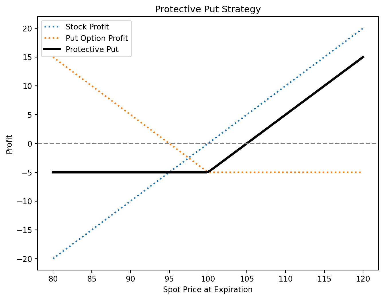
A protective put strategy involves buying a stock (or holding a currently owned stock) and buying a put option for the same stock. This strategy is used to protect against a decline in the stock’s price while allowing for participation in any upside. It guarantees a minimum selling price (the strike price of the put) for the stock until the put’s expiration, effectively setting a floor on the potential losses without capping the potential gains.

Code

# Parameters for the protective put strategy
spot_prices = np.linspace(80, 120, 100)  # Range of spot prices
S0 = 100  # Initial stock price
K = 100  # Strike price of the put option
premium_put = 5  # Premium paid for the put option
initial_investment = S0 + premium_put  # Total initial investment including the put premium

# Profit calculations for protective put
stock_profit = spot_prices - S0  # Profit from the stock alone
put_option_profit = np.maximum(K - spot_prices, 0) - premium_put  # Profit from the long put option
protective_put_profit = stock_profit + put_option_profit  # Total profit from the protective put strategy

# Create the figure
fig = go.Figure()

# Add traces for the individual components' profits
fig.add_trace(
    go.Scatter(
        x=spot_prices,
        y=stock_profit,
        mode="lines",
        name="Stock Profit",
        line=dict(width=2, dash='dot'),
        hovertemplate="Spot Price: %{x:.0f}<br>Profit: %{y:.0f}<extra></extra>",
    )
)
fig.add_trace(
    go.Scatter(
        x=spot_prices,
        y=put_option_profit,
        mode="lines",
        name="Put Option Profit",
        line=dict(width=2, dash='dot'),
        hovertemplate="Spot Price: %{x:.0f}<br>Profit: %{y:.0f}<extra></extra>",
    )
)

# Add trace for the protective put net profit
fig.add_trace(
    go.Scatter(
        x=spot_prices,
        y=protective_put_profit,
        mode="lines",
        name="Protective Put",
        line=dict(width=4),
        hovertemplate="Spot Price: %{x:.0f}<br>Net Profit: %{y:.0f}<extra></extra>",
    )
)

# Horizontal line at profit = 0 for reference, adjusted for the initial investment
fig.add_hline(y=0, line_dash="dash", line_color="black")

# Layout adjustments for clarity
fig.update_layout(
    title="Protective Put Strategy",
    xaxis_title="Spot Price at Expiration",
    yaxis_title="Profit",
    legend_title="Component",
)

# Show the figure
fig.show()

6.2.2 Covered Call

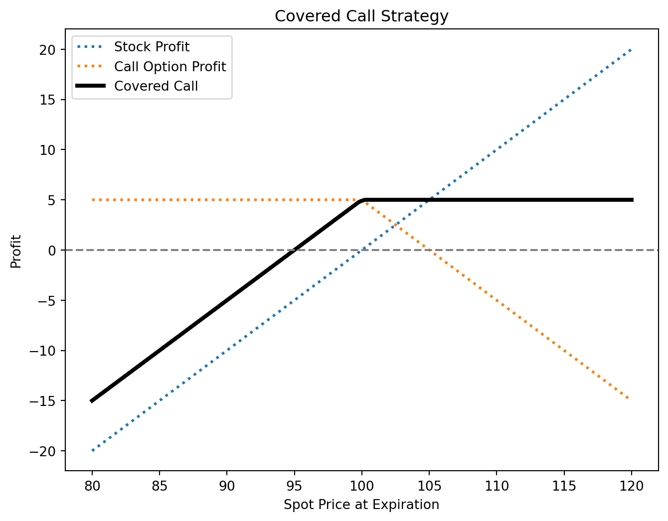
A covered call strategy involves owning a stock and selling a call option on that stock. This strategy is aimed at generating additional income from the option premium, which can enhance the overall returns on the stock, especially in flat or slightly bullish markets. It limits the upside potential to the strike price of the sold call but provides premium income that offers some protection against a decline in the stock’s price.

Code

# Parameters for the covered call strategy
spot_prices = np.linspace(80, 120, 100)  # Range of spot prices
S0 = 100  # Initial stock price
K = 100  # Strike price of the call option
premium_call = 5  # Premium received for the call option

# Profit calculations for covered call
stock_profit = spot_prices - S0  # Profit from the stock alone
call_option_profit = np.where(spot_prices > K, K - spot_prices, 0) + premium_call  # Profit from the short call option
covered_call_profit = stock_profit + call_option_profit  # Total profit from the covered call strategy

# Create the figure
fig = go.Figure()

# Add traces for the individual components' profits
fig.add_trace(
    go.Scatter(
        x=spot_prices,
        y=stock_profit,
        mode="lines",
        name="Stock Profit",
        line=dict(width=2, dash='dot'),
        hovertemplate="Spot Price: %{x:.0f}<br>Profit: %{y:.0f}<extra></extra>",
    )
)
fig.add_trace(
    go.Scatter(
        x=spot_prices,
        y=call_option_profit,
        mode="lines",
        name="Call Option Profit",
        line=dict(width=2, dash='dot'),
        hovertemplate="Spot Price: %{x:.0f}<br>Profit: %{y:.0f}<extra></extra>",
    )
)

# Add trace for the covered call net profit
fig.add_trace(
    go.Scatter(
        x=spot_prices,
        y=covered_call_profit,
        mode="lines",
        name="Covered Call",
        line=dict(width=4),
        hovertemplate="Spot Price: %{x:.0f}<br>Net Profit: %{y:.0f}<extra></extra>",
    )
)

# Horizontal line at profit = 0 for reference
fig.add_hline(y=0, line_dash="dash", line_color="black")

# Layout adjustments for clarity
fig.update_layout(
    title="Covered Call Strategy",
    xaxis_title="Spot Price at Expiration",
    yaxis_title="Profit",
    legend_title="Component",
)

# Show the figure
fig.show()

6.3 Option Spreads

Option spread strategies involve holding two or more options of the same type simultaneously to capitalize on movements in the underlying asset’s price. These strategies can be tailored to reflect various market outlooks, from bullish to bearish or even neutral.

6.3.1 Bull Spread Strategy

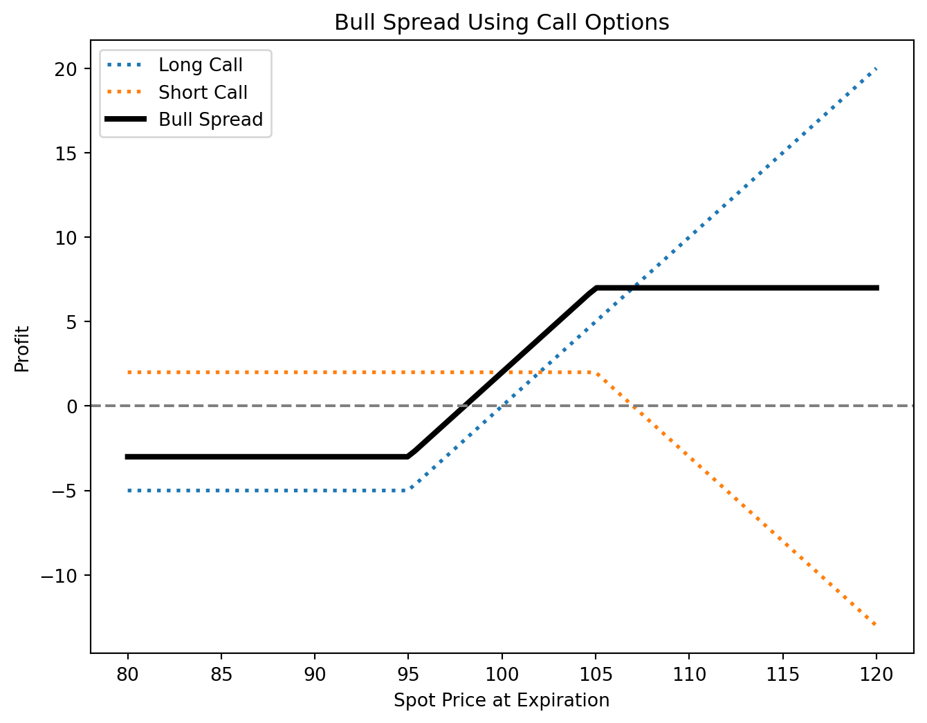
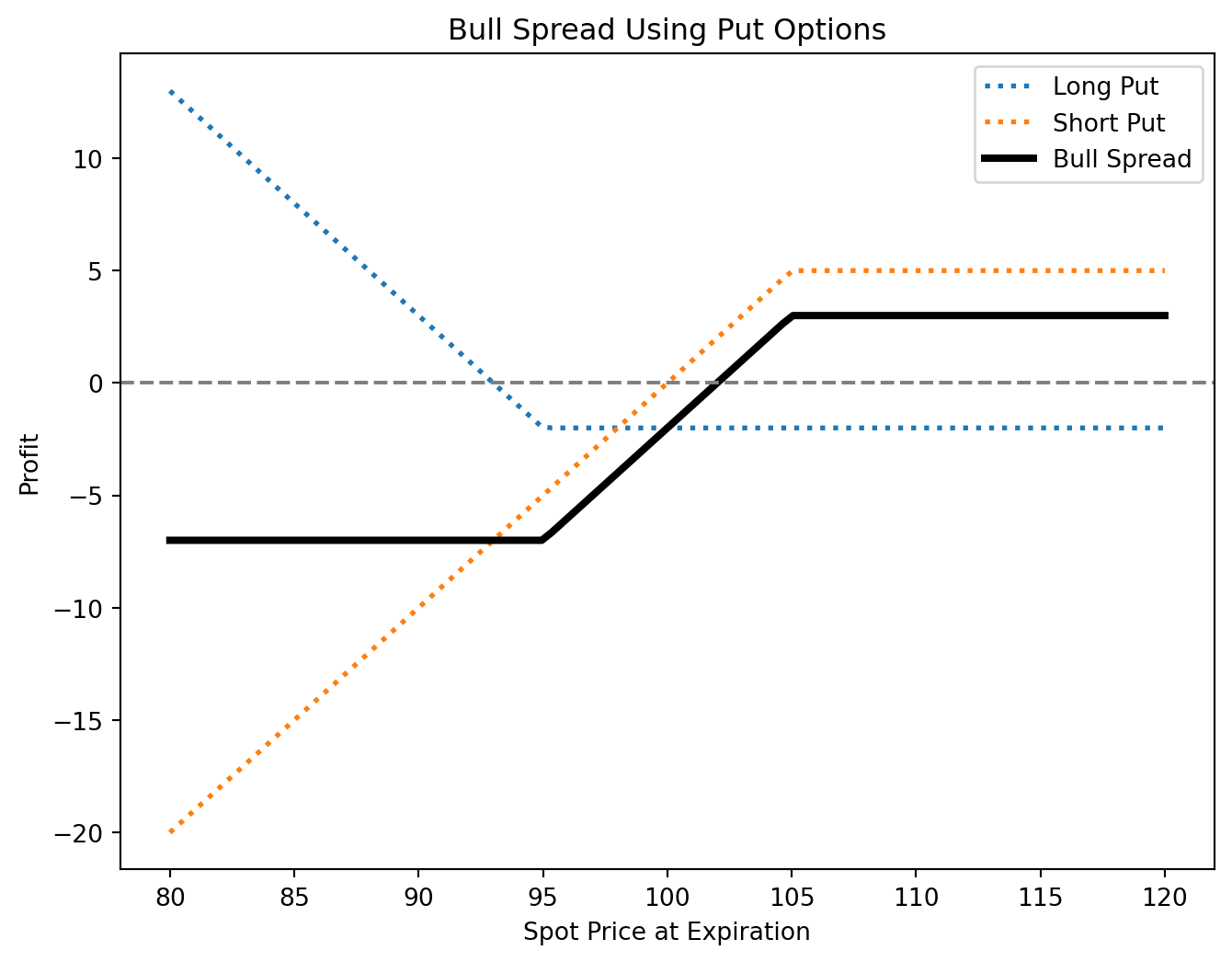
A bull spread is a strategy used when an investor expects a moderate increase in the price of the underlying asset. It can be constructed using either calls or puts.

Using Calls (Call Bull Spread)

Position: Buy a call option with a lower strike price and sell another call option with a higher strike price. Both options share the same expiration date.
Profit Potential: Maximum profit is limited to the difference between the two strike prices minus the net premium paid.
Risk: Limited to the net premium paid for the spread.
Break-even Point: Lower strike price + net premium paid.

Code

# Parameters for the bull spread strategy
spot_prices = np.linspace(80, 120, 100)  # Range of spot prices
K1 = 95  # Strike price of the long call option
K2 = 105  # Strike price of the short call option
premium_long = 5  # Premium paid for the long call
premium_short = 2  # Premium received for the short call

# Profit calculations
long_call_profit = np.maximum(spot_prices - K1, 0) - premium_long
short_call_profit = -(np.maximum(spot_prices - K2, 0) - premium_short)
bull_spread_profit = long_call_profit + short_call_profit  # Net profit of the bull spread

# Create the figure
fig = go.Figure()

# Add traces for the individual option profits
fig.add_trace(
    go.Scatter(
        x=spot_prices,
        y=long_call_profit,
        mode="lines",
        name="Long Call",
        line=dict(width=3, dash='dot'),
        hovertemplate="Spot Price: %{x:.0f}<br>Profit: %{y:.0f}<extra></extra>",
    )
)
fig.add_trace(
    go.Scatter(
        x=spot_prices,
        y=short_call_profit,
        mode="lines",
        name="Short Call",
        line=dict(width=3, dash='dot'),
        hovertemplate="Spot Price: %{x:.0f}<br>Profit: %{y:.0f}<extra></extra>",
    )
)

# Add trace for the bull spread net profit
fig.add_trace(
    go.Scatter(
        x=spot_prices,
        y=bull_spread_profit,
        mode="lines",
        name="Bull Spread",
        line=dict(width=4),
        hovertemplate="Spot Price: %{x:.0f}<br>Net Profit: %{y:.0f}<extra></extra>",
    )
)

# Horizontal line at profit = 0 for reference
fig.add_hline(y=0, line_dash="dash", line_color="black")

# Layout adjustments for clarity
fig.update_layout(
    title="Bull Spread Using Call Options",
    xaxis_title="Spot Price at Expiration",
    yaxis_title="Profit",
    legend_title="Component",
)

# Show the figure
fig.show()

Using Puts (Put Bull Spread)

Position: Buy a put option with a higher strike price and sell another put option with a lower strike price, both having the same expiration date.
Profit Potential: Maximum profit is limited to the difference between the strike prices minus the net premium paid.
Risk: Limited to the net premium paid for the spread.
Break-even Point: Higher strike price - net premium paid.

Code

# Parameters for the bull spread strategy using put options
spot_prices = np.linspace(80, 120, 100)  # Range of spot prices
K1 = 95  # Strike price of the long put option (lower strike)
K2 = 105  # Strike price of the short put option (higher strike)
premium_long = 2  # Premium paid for the long put
premium_short = 5  # Premium received for the short put

# Profit calculations
long_put_profit = np.maximum(K1 - spot_prices, 0) - premium_long
short_put_profit = -(np.maximum(K2 - spot_prices, 0) - premium_short)
bull_spread_profit = long_put_profit + short_put_profit  # Net profit of the bull spread using put options

# Create the figure
fig = go.Figure()

# Add traces for the individual option profits
fig.add_trace(
    go.Scatter(
        x=spot_prices,
        y=long_put_profit,
        mode="lines",
        name="Long Put",
        line=dict(width=3, dash='dot'),
        hovertemplate="Spot Price: %{x:.0f}<br>Profit: %{y:.0f}<extra></extra>",
    )
)
fig.add_trace(
    go.Scatter(
        x=spot_prices,
        y=short_put_profit,
        mode="lines",
        name="Short Put",
        line=dict(width=3, dash='dot'),
        hovertemplate="Spot Price: %{x:.0f}<br>Profit: %{y:.0f}<extra></extra>",
    )
)

# Add trace for the bull spread net profit
fig.add_trace(
    go.Scatter(
        x=spot_prices,
        y=bull_spread_profit,
        mode="lines",
        name="Bull Spread",
        line=dict(width=4),
        hovertemplate="Spot Price: %{x:.0f}<br>Net Profit: %{y:.0f}<extra></extra>",
    )
)

# Horizontal line at profit = 0 for reference
fig.add_hline(y=0, line_dash="dash", line_color="black")

# Layout adjustments for clarity
fig.update_layout(
    title="Bull Spread Using Put Options",
    xaxis_title="Spot Price at Expiration",
    yaxis_title="Profit",
    legend_title="Component",
)

# Show the figure
fig.show()

6.3.2 Bear Spread Strategy

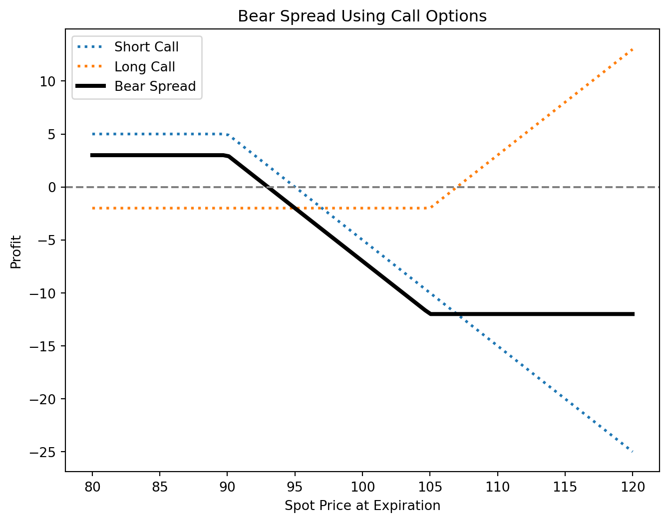
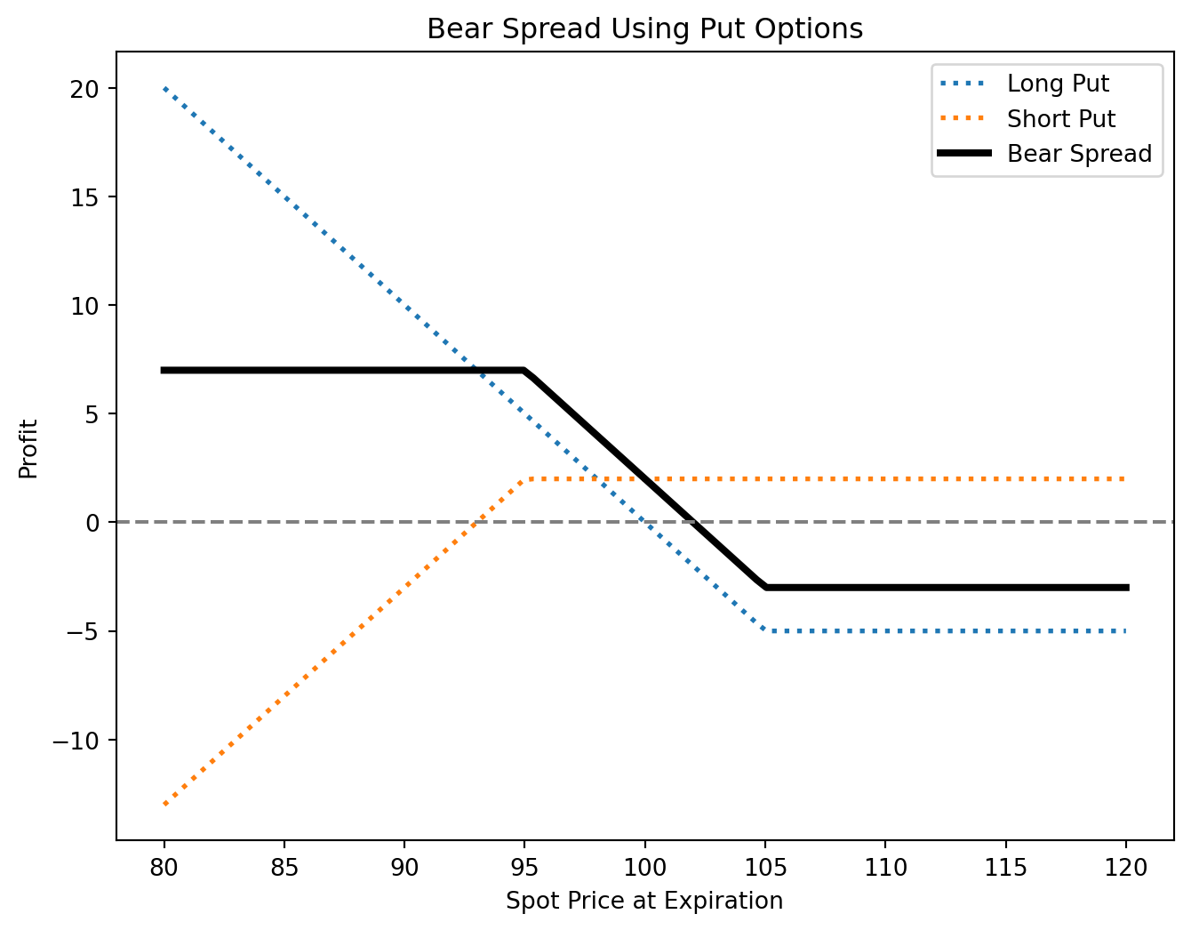
A bear spread is used when an investor expects a moderate decline in the price of the underlying asset. Similar to the bull spread, it can be executed using calls or puts.

Using Calls (Call Bear Spread)

Position: Buy a call option with a higher strike price and sell another call option with a lower strike price, both having the same expiration date.
Profit Potential: Maximum profit is limited to the net premium received for the spread.
Risk: Limited to the difference between the strike prices minus the net premium received.
Break-even Point: Lower strike price + net premium received.

Code

# Parameters for the bear spread strategy using call options
spot_prices = np.linspace(80, 120, 100)  # Range of spot prices
K1 = 90  # Strike price of the short call option (lower strike)
K2 = 105  # Strike price of the long call option (higher strike)
premium_short = 5  # Premium received for the short call
premium_long = 2  # Premium paid for the long call

# Profit calculations for bear spread using call options
short_call_profit = -(np.maximum(spot_prices - K1, 0) - premium_short)
long_call_profit = np.maximum(spot_prices - K2, 0) - premium_long
bear_spread_profit = short_call_profit + long_call_profit  # Net profit of the bear spread

# Create the figure
fig = go.Figure()

# Add traces for the individual option profits
fig.add_trace(
    go.Scatter(
        x=spot_prices,
        y=short_call_profit,
        mode="lines",
        name="Short Call",
        line=dict(width=3, dash='dot'),
        hovertemplate="Spot Price: %{x:.0f}<br>Profit: %{y:.0f}<extra></extra>",
    )
)
fig.add_trace(
    go.Scatter(
        x=spot_prices,
        y=long_call_profit,
        mode="lines",
        name="Long Call",
        line=dict(width=3, dash='dot'),
        hovertemplate="Spot Price: %{x:.0f}<br>Profit: %{y:.0f}<extra></extra>",
    )
)

# Add trace for the bear spread net profit
fig.add_trace(
    go.Scatter(
        x=spot_prices,
        y=bear_spread_profit,
        mode="lines",
        name="Bear Spread",
        line=dict(width=4),
        hovertemplate="Spot Price: %{x:.0f}<br>Net Profit: %{y:.0f}<extra></extra>",
    )
)

# Horizontal line at profit = 0 for reference
fig.add_hline(y=0, line_dash="dash", line_color="black")

# Layout adjustments for clarity
fig.update_layout(
    title="Bear Spread Using Call Options",
    xaxis_title="Spot Price at Expiration",
    yaxis_title="Profit",
    legend_title="Component",
)

# Show the figure
fig.show()

Using Puts (Put Bear Spread)

Position: Buy a put option with a higher strike price and sell another put option with a lower strike price, both having the same expiration date.
Profit Potential: Maximum profit is limited to the net premium received for the spread.
Risk: Limited to the difference between the strike prices minus the net premium received.
Break-even Point: Higher strike price - net premium received.

Code

# Parameters for the bear spread strategy using put options
spot_prices = np.linspace(80, 120, 100)  # Range of spot prices
K1 = 105  # Strike price of the long put option (higher strike)
K2 = 95  # Strike price of the short put option (lower strike)
premium_long = 5  # Premium paid for the long put
premium_short = 2  # Premium received for the short put

# Profit calculations for bear spread using put options
long_put_profit = np.maximum(K1 - spot_prices, 0) - premium_long
short_put_profit = -(np.maximum(K2 - spot_prices, 0) - premium_short)
bear_spread_profit = long_put_profit + short_put_profit  # Net profit of the bear spread

# Create the figure
fig = go.Figure()

# Add traces for the individual option profits
fig.add_trace(
    go.Scatter(
        x=spot_prices,
        y=long_put_profit,
        mode="lines",
        name="Long Put",
        line=dict(width=3, dash='dot'),
        hovertemplate="Spot Price: %{x:.0f}<br>Profit: %{y:.0f}<extra></extra>",
    )
)
fig.add_trace(
    go.Scatter(
        x=spot_prices,
        y=short_put_profit,
        mode="lines",
        name="Short Put",
        line=dict(width=3, dash='dot'),
        hovertemplate="Spot Price: %{x:.0f}<br>Profit: %{y:.0f}<extra></extra>",
    )
)

# Add trace for the bear spread net profit
fig.add_trace(
    go.Scatter(
        x=spot_prices,
        y=bear_spread_profit,
        mode="lines",
        name="Bear Spread",
        line=dict(width=4),
        hovertemplate="Spot Price: %{x:.0f}<br>Net Profit: %{y:.0f}<extra></extra>",
    )
)

# Horizontal line at profit = 0 for reference
fig.add_hline(y=0, line_dash="dash", line_color="black")

# Layout adjustments for clarity
fig.update_layout(
    title="Bear Spread Using Put Options",
    xaxis_title="Spot Price at Expiration",
    yaxis_title="Profit",
    legend_title="Component",
)

# Show the figure
fig.show()

6.3.3 Butterfly Spread Strategy

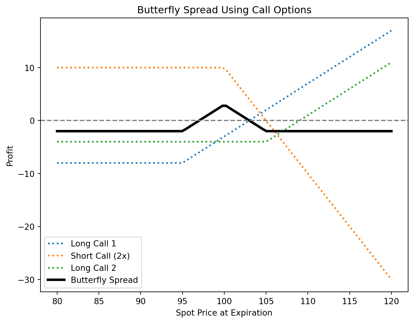
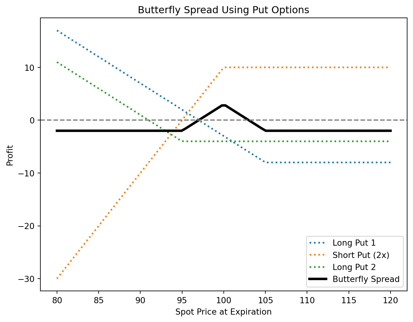
The butterfly spread is a neutral option strategy that is used when an investor expects little to no movement in the underlying asset’s price. It can be constructed using either calls or puts and involves both buying and selling options at three different strike prices.

Using Calls (Call Butterfly Spread)

Position:
- Buy one call option at a lower strike price (A).
- Sell two call options at a middle strike price (B).
- Buy one call option at a higher strike price (C).
- All options have the same expiration date, and the strike prices are equidistant.
Profit Potential: Maximum profit is achieved if the underlying asset’s price is equal to the middle strike price at expiration. The profit is the difference between the middle and lower (or higher) strike prices minus the net premium paid.
Risk: Limited to the net premium paid to establish the spread.
Break-even Points: There are two break-even points:
- Lower break-even: Lower strike price (A) + net premium paid.
- Upper break-even: Higher strike price (C) - net premium paid.

Code

# Parameters for the butterfly spread strategy using call options
spot_prices = np.linspace(80, 120, 100)  # Range of spot prices
K1 = 95  # Strike price of the first long call option (lower strike)
K2 = 100  # Strike price of the short call options (middle strike)
K3 = 105  # Strike price of the second long call option (higher strike)
premium_long1 = 8  # Premium paid for the first long call
premium_short = 5  # Premium received for each short call (twice for the middle strike)
premium_long2 = 4  # Premium paid for the second long call

# Profit calculations for butterfly spread using call options
long_call1_profit = np.maximum(spot_prices - K1, 0) - premium_long1
short_call_profit = 2 * (-(np.maximum(spot_prices - K2, 0) - premium_short))
long_call2_profit = np.maximum(spot_prices - K3, 0) - premium_long2
butterfly_spread_profit = long_call1_profit + short_call_profit + long_call2_profit  # Net profit of the butterfly spread

# Create the figure
fig = go.Figure()

# Add traces for the individual option profits
fig.add_trace(
    go.Scatter(
        x=spot_prices,
        y=long_call1_profit,
        mode="lines",
        name="Long Call 1",
        line=dict(width=2, dash='dot'),
        hovertemplate="Spot Price: %{x:.0f}<br>Profit: %{y:.0f}<extra></extra>",
    )
)
fig.add_trace(
    go.Scatter(
        x=spot_prices,
        y=short_call_profit,
        mode="lines",
        name="Short Call (2x)",
        line=dict(width=2, dash='dot'),
        hovertemplate="Spot Price: %{x:.0f}<br>Profit: %{y:.0f}<extra></extra>",
    )
)
fig.add_trace(
    go.Scatter(
        x=spot_prices,
        y=long_call2_profit,
        mode="lines",
        name="Long Call 2",
        line=dict(width=2, dash='dot'),
        hovertemplate="Spot Price: %{x:.0f}<br>Profit: %{y:.0f}<extra></extra>",
    )
)

# Add trace for the butterfly spread net profit
fig.add_trace(
    go.Scatter(
        x=spot_prices,
        y=butterfly_spread_profit,
        mode="lines",
        name="Butterfly Spread",
        line=dict(width=4),
        hovertemplate="Spot Price: %{x:.0f}<br>Net Profit: %{y:.0f}<extra></extra>",
    )
)

# Horizontal line at profit = 0 for reference
fig.add_hline(y=0, line_dash="dash", line_color="black")

# Layout adjustments for clarity
fig.update_layout(
    title="Butterfly Spread Using Call Options",
    xaxis_title="Spot Price at Expiration",
    yaxis_title="Profit",
    legend_title="Component",
)

# Show the figure
fig.show()

Using Puts (Put Butterfly Spread)

Position:
- Buy one put option at a higher strike price (A).
- Sell two put options at a middle strike price (B).
- Buy one put option at a lower strike price (C).
- All options have the same expiration date, and the strike prices are equidistant.
Profit Potential: Maximum profit is similar to the call butterfly and is achieved if the underlying’s price equals the middle strike price at expiration.
Risk: Limited to the net premium paid for the spread.
Break-even Points: Identical in concept to the call butterfly, adjusted for the put options’ strike prices.

Code

# Parameters for the butterfly spread strategy using put options
spot_prices = np.linspace(80, 120, 100)  # Range of spot prices
K1 = 105  # Strike price of the first long put option (higher strike)
K2 = 100  # Strike price of the short put options (middle strike)
K3 = 95  # Strike price of the second long put option (lower strike)
premium_long1 = 8  # Premium paid for the first long put
premium_short = 5  # Premium received for each short put (twice for the middle strike)
premium_long2 = 4  # Premium paid for the second long put

# Profit calculations for butterfly spread using put options
long_put1_profit = np.maximum(K1 - spot_prices, 0) - premium_long1
short_put_profit = 2 * (-(np.maximum(K2 - spot_prices, 0) - premium_short))
long_put2_profit = np.maximum(K3 - spot_prices, 0) - premium_long2
butterfly_spread_profit = long_put1_profit + short_put_profit + long_put2_profit  # Net profit of the butterfly spread

# Create the figure
fig = go.Figure()

# Add traces for the individual option profits
fig.add_trace(
    go.Scatter(
        x=spot_prices,
        y=long_put1_profit,
        mode="lines",
        name="Long Put 1",
        line=dict(width=2, dash='dot'),
        hovertemplate="Spot Price: %{x:.0f}<br>Profit: %{y:.0f}<extra></extra>",
    )
)
fig.add_trace(
    go.Scatter(
        x=spot_prices,
        y=short_put_profit,
        mode="lines",
        name="Short Put (2x)",
        line=dict(width=2, dash='dot'),
        hovertemplate="Spot Price: %{x:.0f}<br>Profit: %{y:.0f}<extra></extra>",
    )
)
fig.add_trace(
    go.Scatter(
        x=spot_prices,
        y=long_put2_profit,
        mode="lines",
        name="Long Put 2",
        line=dict(width=2, dash='dot'),
        hovertemplate="Spot Price: %{x:.0f}<br>Profit: %{y:.0f}<extra></extra>",
    )
)

# Add trace for the butterfly spread net profit
fig.add_trace(
    go.Scatter(
        x=spot_prices,
        y=butterfly_spread_profit,
        mode="lines",
        name="Butterfly Spread",
        line=dict(width=4),
        hovertemplate="Spot Price: %{x:.0f}<br>Net Profit: %{y:.0f}<extra></extra>",
    )
)

# Horizontal line at profit = 0 for reference
fig.add_hline(y=0, line_dash="dash", line_color="black")

# Layout adjustments for clarity
fig.update_layout(
    title="Butterfly Spread Using Put Options",
    xaxis_title="Spot Price at Expiration",
    yaxis_title="Profit",
    legend_title="Component",
)

# Show the figure
fig.show()

6.3.4 Key Characteristics of Option Spreads

Market Outlook: Bull spreads are used when expecting a moderate price increase, while bear spreads are for a moderate price decrease. Butterfly spread is best suited for markets expected to be stable or within a specific range.
Risk and Reward: Bull and bear spreads strategies offer limited risk and reward, making them attractive for traders with a specific market view and risk tolerance. Butterfly spreado ffers a high reward-to-risk ratio if the market remains stable but with limited profit potential outside the narrow price range.
Cost Efficiency: Spreads can be cost-effective ways to gain market exposure compared to outright option purchases.
Flexibility: Investors can adjust the width of the spread and the strike prices to manage the risk-reward ratio according to their market outlook and risk appetite.

Calendar Spreads

Calendar spreads, also known as time or horizontal spreads, involve options of the same underlying asset, strike price, but different expiration dates. They capitalize on the difference in time decay rates (theta) between options. Typically, a calendar spread is constructed by selling a short-term option and buying a longer-term option of the same type (call or put).

For more information check, e.g., tastylive

6.4 Option Combinations

Option combinations involve two or more options of different types. It allow traders and investors to express complex market views and hedge positions in ways that single option positions cannot. This section covers four popular option combination strategies: straddles, strangles, strips, and straps.

6.4.1 Straddles

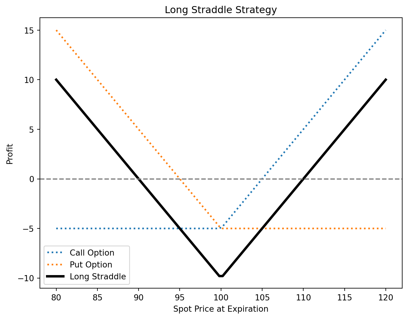
A straddle involves buying or selling both a call and a put option with the same strike price and expiration date.

Long Straddle

A long straddle is created by buying both a call and a put option. It is a bet on volatility without taking a directional stance. Traders expect the underlying asset to move significantly, but they are unsure in which direction. The maximum loss is limited to the total premium paid for both options, while the profit potential is unlimited if the underlying moves significantly in either direction.

Code

# Parameters for the long straddle strategy
spot_prices = np.linspace(80, 120, 100)  # Range of spot prices
K = 100  # Strike price for both the call and put options
premium_call = 5  # Premium paid for the call option
premium_put = 5 # Premium paid for the put option

# Profit calculations for long straddle
call_profit = np.maximum(spot_prices - K, 0) - premium_call
put_profit = np.maximum(K - spot_prices, 0) - premium_put
long_straddle_profit = call_profit + put_profit  # Net profit of the long straddle

# Create the figure
fig = go.Figure()

# Add traces for the individual option profits
fig.add_trace(
    go.Scatter(
        x=spot_prices,
        y=call_profit,
        mode="lines",
        name="Call Option",
        line=dict(width=2, dash='dot'),
        hovertemplate="Spot Price: %{x:.0f}<br>Profit: %{y:.0f}<extra></extra>",
    )
)
fig.add_trace(
    go.Scatter(
        x=spot_prices,
        y=put_profit,
        mode="lines",
        name="Put Option",
        line=dict(width=2, dash='dot'),
        hovertemplate="Spot Price: %{x:.0f}<br>Profit: %{y:.0f}<extra></extra>",
    )
)

# Add trace for the long straddle net profit
fig.add_trace(
    go.Scatter(
        x=spot_prices,
        y=long_straddle_profit,
        mode="lines",
        name="Long Straddle",
        line=dict(width=4),
        hovertemplate="Spot Price: %{x:.0f}<br>Net Profit: %{y:.0f}<extra></extra>",
    )
)

# Horizontal line at profit = 0 for reference
fig.add_hline(y=0, line_dash="dash", line_color="black")

# Layout adjustments for clarity
fig.update_layout(
    title="Long Straddle Strategy",
    xaxis_title="Spot Price at Expiration",
    yaxis_title="Profit",
    legend_title="Component",
)

# Show the figure
fig.show()

Short Straddle

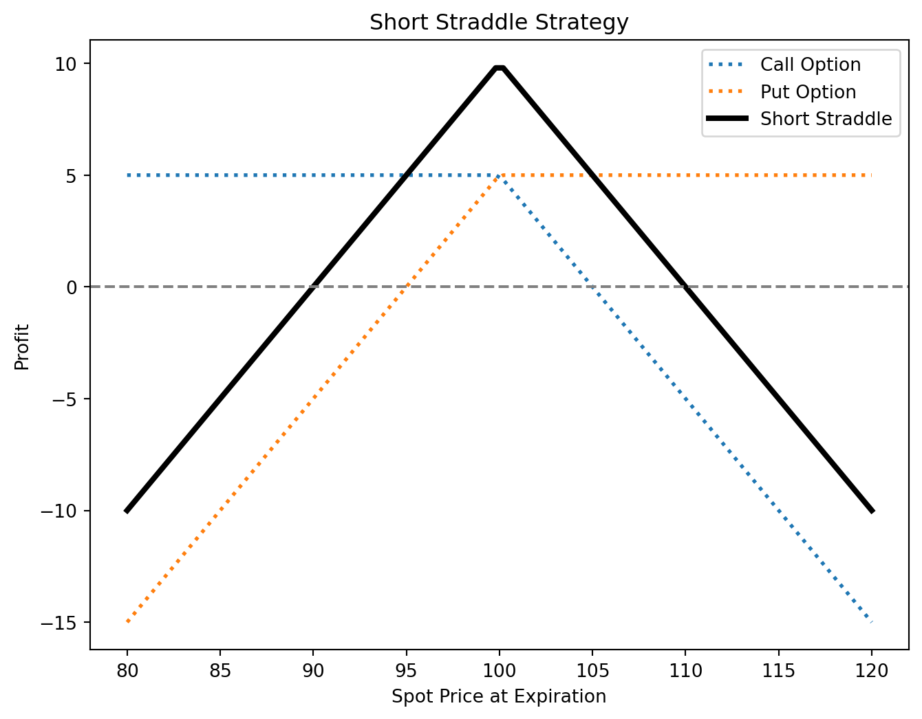
Conversely, a short straddle involves selling a call and a put option. This strategy bets on low market volatility, with the trader expecting the underlying asset to remain stable. The maximum profit is limited to the premiums received, while the risk is theoretically unlimited, as the underlying asset can move significantly in either direction.

Code

# Parameters for the short straddle strategy
spot_prices = np.linspace(80, 120, 100)  # Range of spot prices
K = 100  # Strike price for both the call and put options
premium_call = 5  # Premium received for the call option
premium_put = 5  # Premium received for the put option

# Profit calculations for short straddle
call_profit = np.minimum(K - spot_prices, 0) + premium_call
put_profit = np.minimum(spot_prices - K, 0) + premium_put
short_straddle_profit = call_profit + put_profit  # Net profit of the short straddle

# Create the figure
fig = go.Figure()

# Add traces for the individual option profits
fig.add_trace(
    go.Scatter(
        x=spot_prices,
        y=call_profit,
        mode="lines",
        name="Call Option",
        line=dict(width=2, dash='dot'),
        hovertemplate="Spot Price: %{x:.0f}<br>Profit: %{y:.0f}<extra></extra>",
    )
)
fig.add_trace(
    go.Scatter(
        x=spot_prices,
        y=put_profit,
        mode="lines",
        name="Put Option",
        line=dict(width=2, dash='dot'),
        hovertemplate="Spot Price: %{x:.0f}<br>Profit: %{y:.0f}<extra></extra>",
    )
)

# Add trace for the short straddle net profit
fig.add_trace(
    go.Scatter(
        x=spot_prices,
        y=short_straddle_profit,
        mode="lines",
        name="Short Straddle",
        line=dict(width=4),
        hovertemplate="Spot Price: %{x:.0f}<br>Net Profit: %{y:.0f}<extra></extra>",
    )
)

# Horizontal line at profit = 0 for reference
fig.add_hline(y=0, line_dash="dash", line_color="black")

# Layout adjustments for clarity
fig.update_layout(
    title="Short Straddle Strategy",
    xaxis_title="Spot Price at Expiration",
    yaxis_title="Profit",
    legend_title="Component",
)

# Show the figure
fig.show()

6.4.2 Strangles

A strangle is similar to a straddle but involves options with different strike prices. Typically, the call option has a higher strike price than the put.

Long Strangle

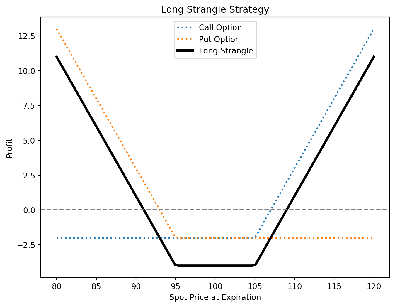
A long strangle is less expensive than a long straddle due to the options being out of the money. It requires a larger move in the underlying asset’s price to be profitable but still benefits from significant volatility without a clear directional bias. The maximum loss is limited to the total premium paid.

Code

# Parameters for the long strangle strategy
spot_prices = np.linspace(80, 120, 100)  # Range of spot prices
K_call = 105  # Strike price of the call option (higher strike)
K_put = 95  # Strike price of the put option (lower strike)
premium_call = 2  # Premium paid for the call option
premium_put = 2  # Premium paid for the put option

# Profit calculations for long strangle
call_profit = np.maximum(spot_prices - K_call, 0) - premium_call
put_profit = np.maximum(K_put - spot_prices, 0) - premium_put
long_strangle_profit = call_profit + put_profit  # Net profit of the long strangle

# Create the figure
fig = go.Figure()

# Add traces for the individual option profits
fig.add_trace(
    go.Scatter(
        x=spot_prices,
        y=call_profit,
        mode="lines",
        name="Call Option",
        line=dict(width=2, dash='dot'),
        hovertemplate="Spot Price: %{x:.0f}<br>Profit: %{y:.0f}<extra></extra>",
    )
)
fig.add_trace(
    go.Scatter(
        x=spot_prices,
        y=put_profit,
        mode="lines",
        name="Put Option",
        line=dict(width=2, dash='dot'),
        hovertemplate="Spot Price: %{x:.0f}<br>Profit: %{y:.0f}<extra></extra>",
    )
)

# Add trace for the long strangle net profit
fig.add_trace(
    go.Scatter(
        x=spot_prices,
        y=long_strangle_profit,
        mode="lines",
        name="Long Strangle",
        line=dict(width=4),
        hovertemplate="Spot Price: %{x:.0f}<br>Net Profit: %{y:.0f}<extra></extra>",
    )
)

# Horizontal line at profit = 0 for reference
fig.add_hline(y=0, line_dash="dash", line_color="black")

# Layout adjustments for clarity
fig.update_layout(
    title="Long Strangle Strategy",
    xaxis_title="Spot Price at Expiration",
    yaxis_title="Profit",
    legend_title="Component",
)

# Show the figure
fig.show()

Short Strangle

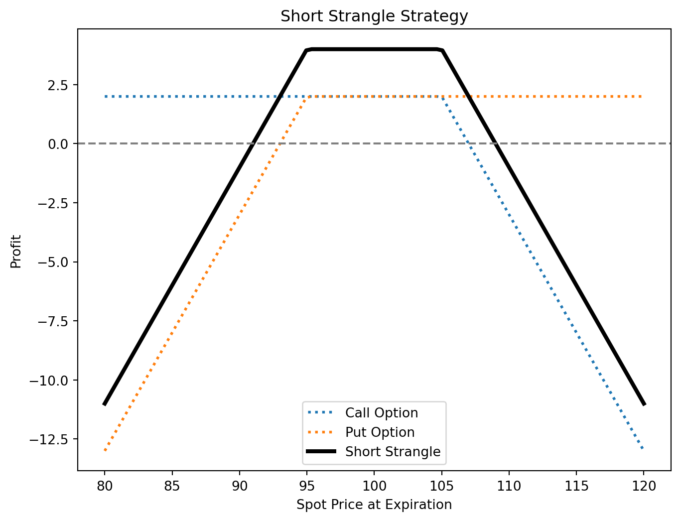
Selling a strangle involves selling an OTM call and an OTM put. This strategy profits from low volatility and time decay. The risk is significant if the underlying moves dramatically, as one of the sold options could become deeply in the money.

Code

# Parameters for the short strangle strategy
spot_prices = np.linspace(80, 120, 100)  # Range of spot prices
K_call = 105  # Strike price of the call option (higher strike)
K_put = 95  # Strike price of the put option (lower strike)
premium_call = 2  # Premium received for the call option
premium_put = 2  # Premium received for the put option

# Profit calculations for short strangle
call_profit = np.minimum(K_call - spot_prices, 0) + premium_call
put_profit = np.minimum(spot_prices - K_put, 0) + premium_put
short_strangle_profit = call_profit + put_profit  # Net profit of the short strangle

# Create the figure
fig = go.Figure()

# Add traces for the individual option profits
fig.add_trace(
    go.Scatter(
        x=spot_prices,
        y=call_profit,
        mode="lines",
        name="Call Option",
        line=dict(width=2, dash='dot'),
        hovertemplate="Spot Price: %{x:.0f}<br>Profit: %{y:.0f}<extra></extra>",
    )
)
fig.add_trace(
    go.Scatter(
        x=spot_prices,
        y=put_profit,
        mode="lines",
        name="Put Option",
        line=dict(width=2, dash='dot'),
        hovertemplate="Spot Price: %{x:.0f}<br>Profit: %{y:.0f}<extra></extra>",
    )
)

# Add trace for the short strangle net profit
fig.add_trace(
    go.Scatter(
        x=spot_prices,
        y=short_strangle_profit,
        mode="lines",
        name="Short Strangle",
        line=dict(width=4),
        hovertemplate="Spot Price: %{x:.0f}<br>Net Profit: %{y:.0f}<extra></extra>",
    )
)

# Horizontal line at profit = 0 for reference
fig.add_hline(y=0, line_dash="dash", line_color="black")

# Layout adjustments for clarity
fig.update_layout(
    title="Short Strangle Strategy",
    xaxis_title="Spot Price at Expiration",
    yaxis_title="Profit",
    legend_title="Component",
)

# Show the figure
fig.show()

6.4.3 Strips and Straps

Strips and straps are modifications of the straddle strategy, offering a directional bias while still betting on volatility.

Strip: A strip consists of buying one call option and two put options with the same strike price and expiration. This strategy bets on volatility but with a bearish outlook, as the additional put provides extra profit if the underlying asset’s price falls.
Strap: A strap involves buying two call options and one put option with the same strike price and expiration. It is similar to a strip but with a bullish outlook, benefiting from an upward move in the underlying asset’s price.

6.4.4 Key Characteristics of Option Combinations

Volatility Sensitivity: All these strategies are sensitive to changes in implied volatility. Long positions in straddles, strangles, strips, and straps benefit from an increase in volatility, while short positions benefit from a decrease.
Directional Bias: Straddles and strangles are primarily non-directional strategies that profit from significant price movements in either direction. Strips and straps introduce a directional bias, offering asymmetric payoffs based on the underlying asset’s movement.
Risk and Reward: The risk-reward profile varies significantly between these strategies. Long positions have limited risk and potentially unlimited reward, while short positions offer limited profit potential with significant risk.
Breakeven Points: These strategies have two breakeven points, one on each side of the underlying asset’s price at entry. The underlying must move beyond these points for long strategies to profit.

6.5 Practice Questions and Problems

What is meant by a protective put? What position in call options is equivalent to a protective put?
Explain two ways in which a bear spread can be created.
When is it appropriate for an investor to purchase a butterfly spread?
What trading strategy creates a reverse calendar spread?
What is the difference between a strangle and a straddle?
A call option with a strike price of $50 costs $2. A put option with a strike price of $45 costs $3. Explain how a strangle can be created from these two options. What is the pattern of profits from the strangle?
Explain how an aggressive bear spread can be created using put options.
Suppose that put options on a stock with strike prices $30 and $35 cost $4 and $7, respectively. How can the options be used to create (a) a bull spread and (b) a bear spread? Draw and explain profit/loss.
An investor believes that there will be a big jump in a stock price, but is uncertain as to the direction. Identify six different strategies the investor can follow and explain the differences among them.